CIBAR: Plotting bar graphs with confidence intervals in Stata
Summarizing data graphically allows to have a quick glance at data of interest. For instance, we may want to assess whether a variable’s mean differs accross different groups. Stata allows to do that easily with grouped bar plots: graph bar dep_var, over(groups). However, to perform statistical inference about group differences, we require a measure of uncertainty (e.g. confidence intervals) around the group means. Without uncertainty measures, we cannot be sure whether a difference in means is in fact due to groups or rather a result of sampling error.1 Hence, optimally, we would invoke Stata’s graph bar with the ci-option. Alas, this option does not exist.
Unsurprisingly, I am not the first looking for bar plots with confidence intervals. As a matter of fact, there are already some user-written Stata packages from the Statistical Software Components (SSC) archive, see e.g. here, that address this issue. However, their syntax is quite different, or produce graphs that look quite different compared to Stata’s graph bar. The UCLA’s Institute for Digital Research and Education provides a very helpful recipe to construct bar graphs that look like those created by Stata. Construction however still requires to compute group means, standard errors, and confidence intervals, setting up a twoway graph, adding some space between the bars, etc. In brief, construction of such bar plots remains rather tedious.
In order to avoid setting up and executing the numerous steps mentioned above whenever I want to visually compare means across groups, I wrote the cibar command, which takes care of all the heavy lifting. cibar’s basic syntax furthermore mimicks graph bar’s quite closely, hence making the transition rather effortless. One can download and install cibar with ssc install cibar.
Heavily drawing from the Institute for Digital Research and Education’s step-by-step guide, cibar essentially works as follows:2
- compute group means and associated standard errors
- derive confidence intervals from means and SEs
- combine means and confidence intervals into a twoway graph
- arrange bars/CIs according to grouping variable, add space between groups, set legends, etc.
Syntax
cibar’s syntax resembles graph bar’s quite closely:
cibar varname [if] [a|f|i|pweights], over(groups) [, options]
The main options consist of:
- level
- confidence level for confidence intervals. Defaults to 95.
- vce
- method to compute standard errors. Defaults to analytic (asymptotic) standard errors. Further options are cluster, bootstrap, and jackknife. Especially bootstrap and jacknife may prove useful when group sizes are small.
Furthermore, there are many graph options (see cibar help file).
Examples
Using Stata’s auto dataset, we can compare prices of US-built and foreign-built cars:
sysuse auto /* load auto data */
cibar price, over(foreign)
Ignoring the fact that the y-axis does not start at 0 (and which behaves the same way with graph bar), we see that on average, foreign cars cost roughly about 400 USD more than US cars (6,000 USD vs. 6,400 USD). However, thanks to the confidence intervals, we see that the average foreign car price lies well within the 95% confidence range of US car prices. Simply put, there is no statictisally significant difference in car prices between US and foreign cars.
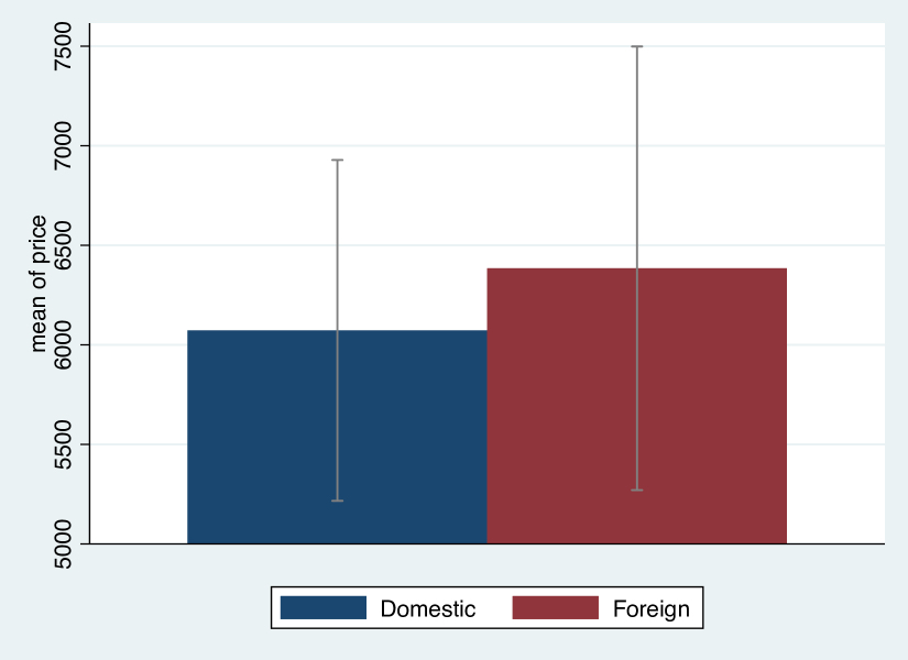
Figure 1: Basic cibar plot
Now, maybe prices do differ between foreign and US cars when breaking the data down into additional groups:
cibar price, over(foreign turn)
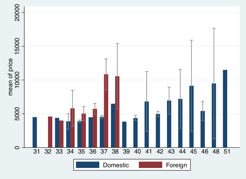
Figure 2: Average car price, jointly by foreign and turn
We notice that there are missing bars for values of turn: clearly, foreign cars do not have turn circles with a diameter larger than 38 feet. Furthermore, comparing foreign and domestic (US) cars with comparable turn circles, foreign cars appear to be substantially more expensive than US cars. Note that some groups consist of only one entry, as some bars display an average price, but no confidence intervals.
Changing the color of the confidence intervals and adding a title to the graph:
cibar price, over(foreign turn) ///
    ciopts(lcolor(red)) ///
    graphopts(title("Price over 'foreign' over 'turn'"))

Figure 3: Average car price, jointly by foreign and turn, coloured confidence intervals
cibar also allows to compute means and confidence intervals for weighted data. Let us inspect the probability of heart attacks in different demographic groups in the US using NHANES data.3 Figure 4 shows that the risk of a heart attack in white women is significantly lower than within white men. We find a similar pattern with African American respondents, however, we cannot tell whether this difference is also statistically significant, as the confidence intervals are rather wide. There is not enough data to investigate the difference in heart attack incidence in repondents of race “other”. Given the missing bar with regard to “other” men, no man of this group has reported a heart attack. Similarly, the extremely wide (analytic) confidence interval suggests very few data on “other” women. As indicated earlier, when dealing with very small groups, confidence intervals derived from analytical standard errors should not be trusted.
webuse total /* load nhanes data */
cibar heartatk, over(sex race)
cibar heartatk [pweight=swgt], over(sex race)
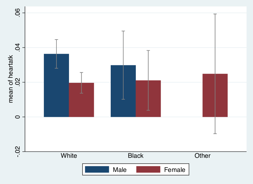
Figure 4: Heart attack incidence, jointly by sex and race, weighted data
-
To be sure, when groups are small, analytical standard errors may be inaccurate and unstable, very sensitive to single cases. Consider bootstrap or jackknife-standard errors instead. ↩︎
-
For more details, look at cibar’s source code, which can be found at https://ideas.repec.org/c/boc/bocode/s457805.html. ↩︎
-
The data is part of Stata’s example dataset nhanes2.dta, and contains variables about respondent heart attack incidence, gender (female, male), race (labelled black, white, and other), and sampling weight. ↩︎