De Metropolis-Hastingis algorithmo
In contrast to OLS and MLE, where parameter estimation essentially boils down to solving something along the lines of , or respectively searching for such that the likelihood is largest, estimating Bayesian models may at first feel like resorting to a black box which mysteriously produces posterior densities . In an attempt to lift this veil of mystery, we will take a look at the Metropolis-Hastings sampler, one of those black boxes used to estimate posterior densities.
In a nutshell, the Metropolis-Hastings algorithm draws random samples from probability distributions .1 To move through the parameter space, the algorithm requires a function which is proportional to the target distribution . At each iteration , the algorithm generates a candidate value from a proposal distribution . To decide whether to accept this value as a draw from ), the algorithm computes the ratio of the current candidate value and the value obtained at the previous iteration (), possibly corrected for asymmetric proposal distributions. If the ratio is larger than or equal to one, is directly accepted as a draw from . If the ratio is smaller than one, the proposal is rejected with a non-zero probability.
To use the MH algorithm for posterior density estimation, first remember Bayes’ theorem: For any continuous parameter and data ,
The Metropolis-Hastings algorithm samples from as follows:
-
generate a candidate value from the proposal distribution . denotes the value at the beginning of iteration .
-
compute the acceptance probability :
with . denotes the probability of producing conditional on the draw of the previous iteration.2
-
generate Unif:
and go back to 1. until convergence to .3
Random walk Metropolis-Hastings
To see how the algorithm explores a posterior density, let’s implement a Metropolis-Hastings sampler in R. Assume we want to investigate the association between biochemistry doctoral students’ characteristics and the number of journal articles they write.4 The characteristics are gender (woman), marital status (married), number of children aged 5 or younger (kid), the prestige of the PhD department (phd), and the count of articles produced by the student’s mentor (mentor). The dependent variable consists of the student’s count of produced journal articles (art), so we model , , with coefficient vector and the covariates described above.
loglik <- function(betastar, y, X) {
  ll <- sum(dpois(y, lambda = exp(X %*% betastar), log = TRUE))
  return(ll)
}
Or, alternatively, write down the log likelihood function
loglik <- function(betastar, y, X) {
  ll <- sum(y * (X %*% betastar) - exp(X %*% betastar) - log(factorial(y)))
  return(ll)
}
We will assume a (multivariate) normal prior for the coefficients, with prior mean vector and prior variance : .
lprior <- function(betastar, b_0, B_0) {
  lp <- dmvnorm(betastar, mean = b_0, sigma = B_0, log = TRUE)
  # requires the package "mvtnorm"
  return(lp)
}
Quite crucially, our sampler requires the jumping density . For simplicity, we start with , that is a random-walk with a step size determined by .
j <- function(beta_t, P) {
  proposal <- mvrnorm(1, beta_t, P)
  return(proposal)
}
With a gaussian jumping distribution centered at the value of the previous proposal, the probability of generating from is equal to generating from . The proportion of these probabilities hence being one, we may omit the correction for asymmetric proposal densities (and in fact use the Metropolis algorithm).
for (t in 2:nsim) {
  # step 1: generate proposal values
  betastar <- j(betasim_rw[t-1,], P)
  # step 2: compute acceptance probability
  r <- exp(loglik(betastar, y, X) -
	   loglik(betasim_rw[t-1,], y, X) +
	   lprior(betastar, b_0, B_0) -
	   lprior(betasim_rw[t-1,], b_0, B_0))
  # step 3: accept/reject
  alpha <- min(r, 1)
  if (runif(1) <= alpha) {
    betasim_rw[t, ] <- betastar
  } else {
    betasim_rw[t, ] <- betasim_rw[t-1, ]
  }
}
Before being able to run the algorithm, we need to specify the starting values of the Markov chain, the mean and variance of the prior , and the step size (the covariance) of the jumping distribution . For simplicity, the algorithm shall start at the value of the maximum likelihood estimates , and use a vague prior with mean and variance .
The element that requires some thought is the step size of the proposal density. If the step size is too large, many candidate values may fall into low-probability regions of the target density, and thus be rejected by the algorithm. Simply put, the Markov chain may not move forward. If the step size is too small however, the algorithm may explore only very slowly. The authors of the R package MCMCpack (Martin, Quinn, and Park 2011) for instance set , with , and being the covariance matrix of the MLE . To keep things simple, we will do the same.
Putting the different pieces together in an R-function and running the algorithm 100,000 times:
## ---- Random-walk Metropolis-Hastings algorithm ----
library(MASS)
library(pscl)
library(mvtnorm)

# ---- random-walk MH sampler ----
rw_metropolis_hastings <- function(y, X, betasim_rw,
				   P,
				   b_0, B_0,
				   nsim) {
  # loglikelihood
  loglik <- function(betastar, y, X) {
    ll <- sum(dpois(y, lambda = exp(X %*% betastar), log = TRUE))
    return(ll)
  }
  # log-prior function
  lprior <- function(betastar, b_0, B_0) {
    lp <- dmvnorm(betastar, mean = b_0, sigma = B_0, log = TRUE)
    # requires the package "mvtnorm"
    return(lp)
  }
  # jumping distribution
  j <- function(beta_t, P) {
    proposal <- mvrnorm(1, beta_t, P)
    return(proposal)
  }
  # sampler
  set.seed(100)
  for (t in 2:nsim) {
    # step 1: generate proposal values
    betastar <- j(betasim_rw[t-1,], P)
    # step 2: compute acceptance probability
    r <- exp(loglik(betastar, y, X) -
	     loglik(betasim_rw[t-1,], y, X) +
	     lprior(betastar, b_0, B_0) -
	     lprior(betasim_rw[t-1,], b_0, B_0))
    # step 3: accept/reject
    alpha <- min(r, 1)
    if (runif(1) <= alpha) {
      betasim_rw[t, ] <- betastar
    } else {
      betasim_rw[t, ] <- betasim_rw[t-1, ]
    }
  }
  return(betasim_rw)
}

# ---- data ----
head(bioChemists, 10)
y <- bioChemists$art
X <- model.matrix(art ~ ., data = bioChemists)
dimnames(X)[[2]] <- c("intercept", "woman", "married", "kid", "phd", "mentor")

# ---- prior mean and variance ----
k <- ncol(X)
b_0 <- vector(mode = "numeric", length = k) # vector values automatically initialized to 0.
B_0 <- diag(rep(10^4, k))

# ---- starting values, step size of jumping distribution ----
inits <- glm(art ~ ., data = bioChemists, family = poisson(link = "log"))

# starting values
beta_start <- coef(inits)

# covariance matrix P for step size of jumping distribution
V <- vcov(inits)
Tmat <- diag(rep(1.1, k))
P <- Tmat %*% solve(solve(B_0) + solve(V)) %*% Tmat

# ---- some housekeeping: results object ----
nsim <- 10^5
betasim_rw <- matrix(beta_start, nrow = nsim, ncol = k, byrow = TRUE)
colnames(betasim_rw) <- colnames(X)

# ---- run algorithm ----
betasim_rw_R <- rw_metropolis_hastings(y, X, betasim_rw,
				       P,
				       b_0, B_0,
				       nsim)
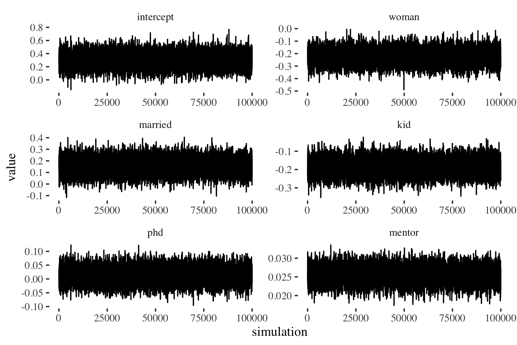
Figure 1: Random-walk MH: Markov chain exploring (p(beta|y, X))

Figure 2: Autocorrelation plots of the random-walk MH draws
We run the random-walk MH algorithm 100,000 times and discard the first 1,000 draws. To rather quickly assess stationarity of the Markov chains, we plot the values generated at each iteration of the MH algorithm separately for each covarate. As we can see in figure 1, the chains seem to have reached their stationary state quite soon, we don’t see the chains wandering around very much.5 The autocorrelation plots (see figure 2) display a rather high correlation between sample draws, indicating a somewhat inefficient sampling scheme.
| estimate | 2.5% | 97.5% | ||||
|---|---|---|---|---|---|---|
| intercept | 0.305 | 0.102 | 0.503 | 0.102 | 0.002 | 0.998 |
| woman | -0.224 | -0.332 | -0.116 | 0.055 | 1.000 | 0.000 |
| married | 0.155 | 0.034 | 0.278 | 0.062 | 0.005 | 0.995 |
| kid | -0.185 | -0.266 | -0.107 | 0.040 | 1.000 | 0.000 |
| phd | 0.013 | -0.037 | 0.065 | 0.026 | 0.317 | 0.683 |
| mentor | 0.025 | 0.021 | 0.029 | 0.002 | 0.000 | 1.000 |
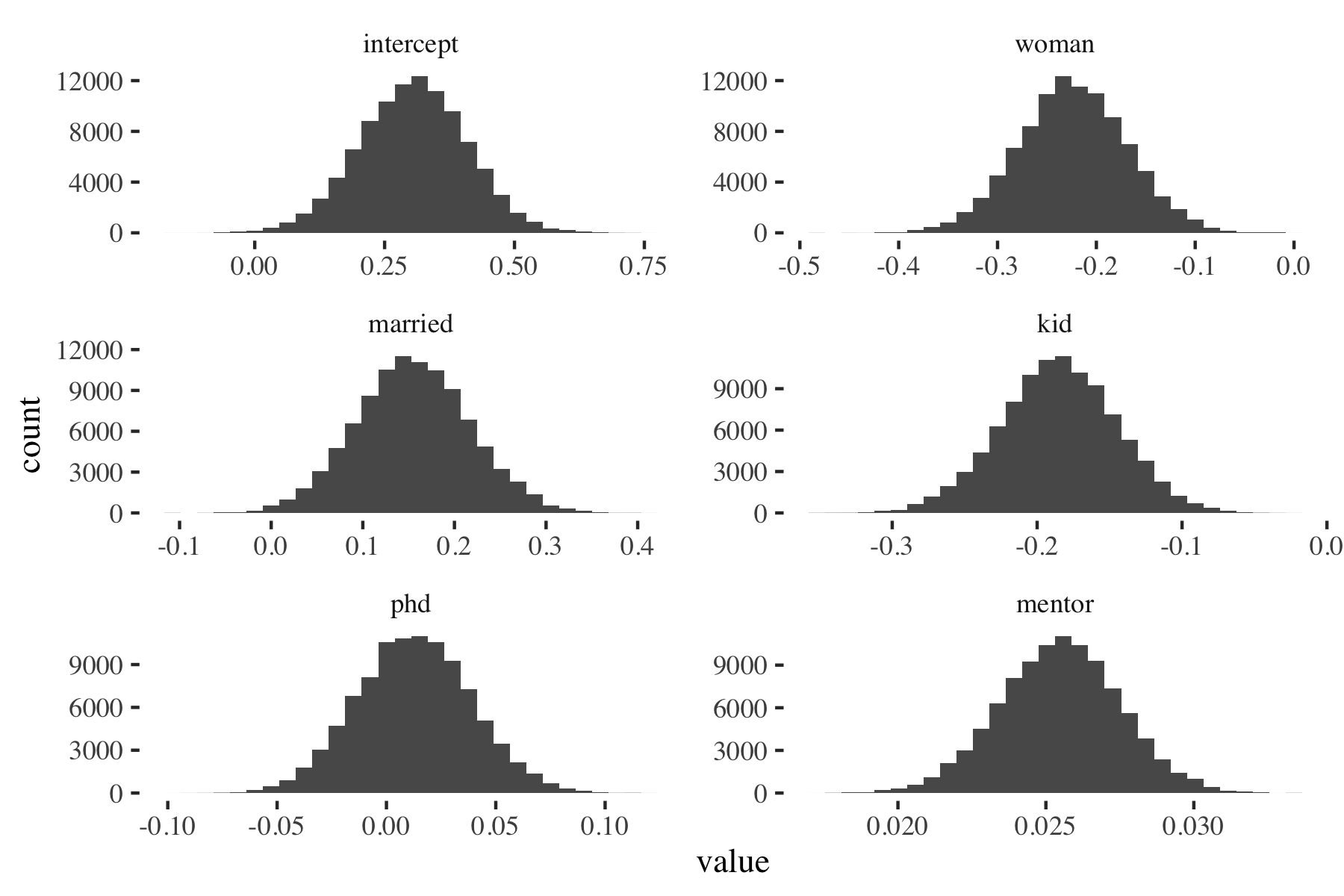
Figure 3: Random-walk MH: Posterior density (p(beta|y, X))
Independent Metropolis-Hastings
As we have seen above, the Metropolis algorithm with random-walk jumping distribution provides quite correlated samples from the posterior. As a matter of fact, the jumping distribution of each candidate is determined by the set of values of the previous iteration. Correlated samples are not an issue per se, the algorithm just needs to run for quite a while to produce a sufficient number of independent draws from the posterior. To avoid the inefficiencies associated with the random-walk, we can implement a jumping distribution that produces independent candidate values.
## ---- Independent Metropolis-Hastings algorithm ----

# ---- independent MH sampler ----
indep_metropolis_hastings <- function(y, X, betasim_indep,
				      beta_1, V_1,
				      b_0, B_0,
				      nsim) {
  # loglikelihood
  loglik <- function(betastar, y, X) {
    ll <- sum(dpois(y, lambda = exp(X %*% betastar), log = TRUE))
    return(ll)
  }
  # log-prior function
  lprior <- function(betastar, b_0, B_0) {
    lp <- dmvnorm(betastar, mean = b_0, sigma = B_0, log = TRUE)
    # requires the package "mvtnorm"
    return(lp)
  }
  # jumping distribution
  j <- function(beta_t, P) {
    proposal <- mvrnorm(1, beta_t, P)
    return(proposal)
  }
  # sampler
  set.seed(100)
  for (t in 2:nsim) {
    # step 1: proposal values
    betastar <- j(beta_1, V_1)
    # step 2: compute acceptance probability,
    # including correction for asymmetric proposal distribution
    r <- exp(loglik(betastar, y, X) -
	     loglik(betasim_indep[t-1,], y, X) +
	     lprior(betastar, b_0, B_0) -
	     lprior(betasim_indep[t-1,], b_0, B_0) +
	     dmvnorm(betasim_indep[t-1,], beta_1, V_1, log = TRUE) -
	     dmvnorm(betastar, beta_1, V_1, log = TRUE))
    # step 3: accept/reject
    alpha <- min(r, 1)
    if (runif(1) <= alpha) {
      betasim_indep[t, ] <- betastar
    } else {
      betasim_indep[t, ] <- betasim_indep[t-1, ]
    }
  }
  return(betasim_indep)
}

# ---- proposal density ----
beta_hat <- coef(inits)
V <- vcov(inits)
k <- length(beta_hat)

# proposal mean and variance
beta_1 <- solve(solve(B_0) + solve(V)) %*% (solve(B_0) %*% b_0 + solve(V) %*% beta_hat)
Tmat <- diag(rep(1.1, k))
V_1 <- Tmat %*% solve(solve(B_0) + solve(V)) %*% Tmat

# ---- some housekeeping: results object ----
nsim <- 10^4
betasim_indep <- matrix(beta_hat, nrow = nsim, ncol = k, byrow = TRUE)
colnames(betasim_indep) <- colnames(X)

# ---- run algorithm ----
betasim_indep_R <- indep_metropolis_hastings(y, X, betasim_indep,
					     beta_1, V_1,
					     b_0, B_0,
					     nsim)
To keep things simple, we will generate candidates from a multivariate normal distribution: .6 Jackman (2009)7 suggests to set to the precision-weighted average and , with . Given that the samples generated by the independent jumping distribution are uncorrelated (see figure 4), we run the algorithm for only 10,000 iterations; the results are (almost) identical (table 2) to those obtained from the random-walk.
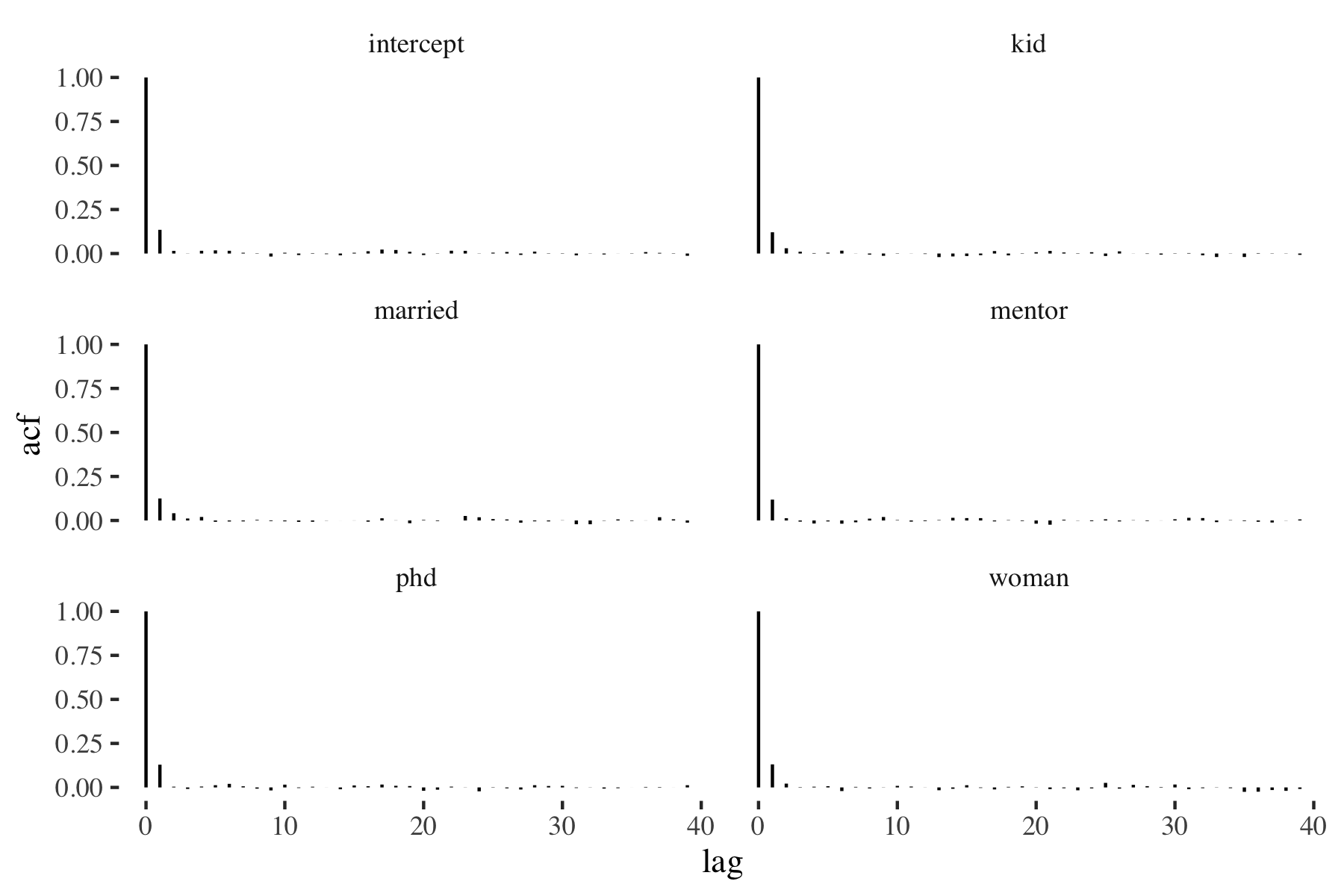
Figure 4: Autocorrelation plots of the independent MH draws
| estimate | 2.5% | 97.5% | ||||
|---|---|---|---|---|---|---|
| intercept | 0.301 | 0.096 | 0.504 | 0.104 | 0.001 | 0.999 |
| woman | -0.224 | -0.334 | -0.117 | 0.056 | 1.000 | 0.000 |
| married | 0.156 | 0.037 | 0.280 | 0.062 | 0.006 | 0.994 |
| kid | -0.185 | -0.264 | -0.107 | 0.040 | 1.000 | 0.000 |
| phd | 0.013 | -0.038 | 0.065 | 0.027 | 0.311 | 0.689 |
| mentor | 0.025 | 0.022 | 0.029 | 0.002 | 0.000 | 1.000 |
Concluding remarks
In this post, we attempted to shed some light on Bayesian estimation algorithms, which at first glance may seem quite arcane. More specifically, we looked at the Metropolis-Hastings algorithm, which at the end of the day is a surprisingly simple and elegant tool to obtain posterior densities. As a matter of fact, the MH algorithm consists of very few building blocks — a likelihood function, a prior density, and a proposal distribution — and works according to the following scheme:
- generate a candidate value.
- compute the ratio of the posterior (likelihood prior) evaluated at the candidate value and the posterior evaluated at the value of the previous iteration
- accept the candidate if the ratio is at least 1, otherwise reject it with a nonzero probability. Continue with step 1.
We have seen that the choice of jumping distribution makes a difference with regard to the sampling efficiency and thus the algorithm’s required run time: Independent proposal densities may for instance allow very efficient (and thus shorter) sampling from the posterior distribution; but only when fitting the target density well. An ill-fitting independent jumping distribution on the other hand might lead to a very high rejection rate and poor exploration of the posterior density. Random-walk proposal distributions alleviate this problem, at the cost of higher autocorrelations.
Last, the above R implementation of the Metropolis-Hastings algorithm takes some time to run the 100,000 respectively 10,000 iterations, even though it already uses vectorized R functions. We will look at a lower-level (and faster) implementation of the MH algorithm in C in another post.
Note: The code used for the above computations can be found at https://git.staudtlex.de/blog/metropolis-hastings-r.
-
See Chib/Greenberg (1995) for more details on the MH algorithm. ↩︎
-
With symmetric proposal distributions, ,
This corresponds to the transition probabilities of the Metropolis algorithm. ↩︎
-
Convergence of MCMC samplers may or may not be discussed in a future post. ↩︎
-
The data frame
bioChemistsis part of Simon Jackman’s R packagepscl. ↩︎ -
Usually, we would additionally run stationarity-related tests such as the Geweke diagnostic, Heidelberger-Welch test for nonstationarity, Raftery-Lewis estimate, and the Gelman-Rubin statistic (when running several algorithms in parallel). ↩︎
-
With this jumping distribution, the probability of obtaining from ( ist fixed) is in general different from obtaining . We correct for these unequal probabilities by including the ratio . ↩︎
-
Jackman, Simon. 2009. Bayesian Analysis for the Social Sciences. Wiley: Chichester. ↩︎